Problem Set: Hillslopes

Problem set / lab (depending on whether “computer lab” = “real lab”) on hillslope diffusion and evolution alongside landsliding. 110 points total

Learning Goals

In this problem set, you will:

• Analyze a small region of southeastern Minnesota using 1-meter LiDAR topography to understand and apply hillslope processes.
• Use slope to identify zones of landsliding vs. hillslope creep.
• Work to understand landslide susceptibility as a function of slope, pore-fluid pressure, and cohesion.
• Use hilltop curvature to estimate the overall landscape erosion rate and project it into the future.

Need a review on QGIS? Look into the prior lab.

1. Angle of repose (15 points)

Based on the analysis of a block on an inclined plane, which is analogous to slip within a continuous medium (like, let’s just say, a hill formed of sand), failure (i.e., slip of the block) will occur at a certain angle. I want you to:

(a) 5 points: Free-body diagram

Set up the free-body diagram for either the block on an inclined plane or the failing continuum.

(b) 5 points: Equation set-up

Write the equation that relates the failure angle to the coefficient of friction, \(\mu\). Show your work.

(c) 5 points: Compute angle of repose

Compute the angle of internal friction, which is equal to the failure angle in the block-on-an-inclined-plane example, for a hill made of sand. The coefficient of internal friction of sand, which is analogous to the frictional coefficinet between the block and plane, is \(\mu = 0.6\). Because this is the angle at which materials will fail, this is the angle that the topography of a cohesionless hill of that material (in this case, sand) will form. Provide the angle of repose, along with your work.

2. Distribution of slope in a landscape governed by fluvial and hillslope processes (20 points)

Here, we’re returning to QGIS where you will use some basic landscape-analysis tools alongside the DEM from the earlier lab exercise. You should feel free to reopen this old exercise and save yourself a bit of time! Otherwise, download the DEM and start fresh.

(a) 10 points: Produce a slope histogram for a portion of this southeastern Minnesota landscape

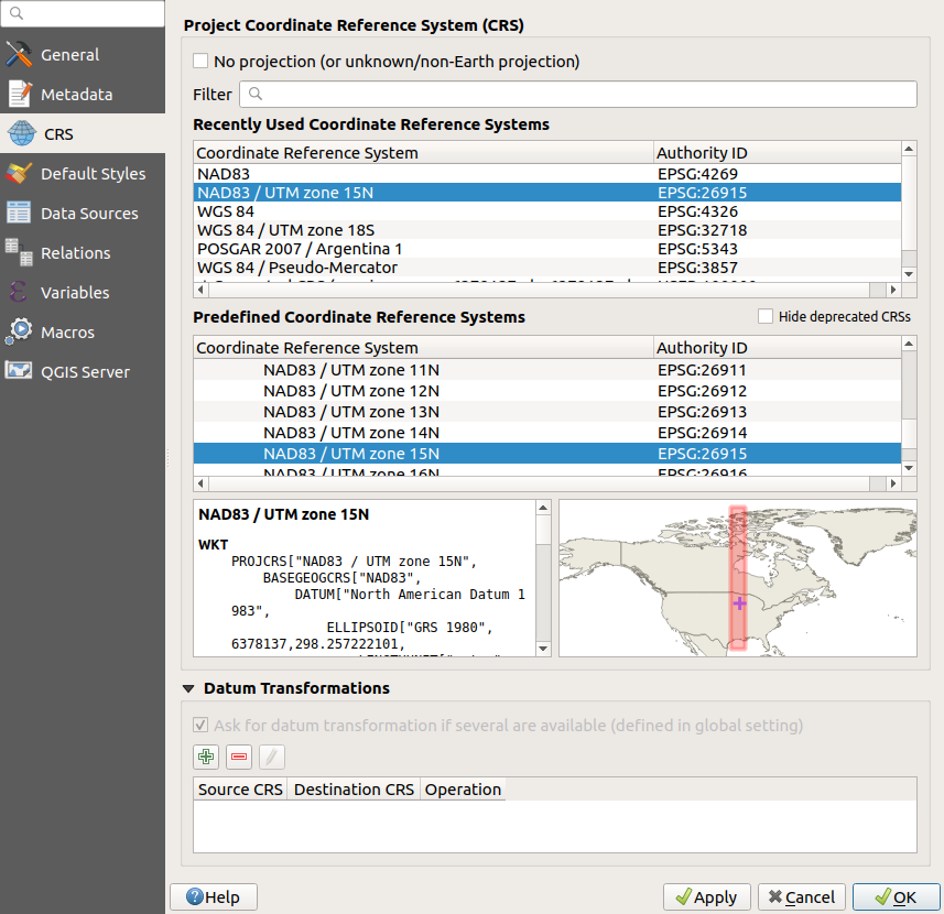
First, import the DEM (if needed) and be sure that your project coordinate system is in UTM 15N with the NAD 83 datum. The EPSG code of the projection is 26915.

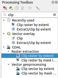
Then, look to the “processing toolbox” to the right. If you cannot see it, go to view → panels → processing toolbox.

You’ll want to become acquainted with this – it holds many useful tools for computing and comparing geographic and geomorphic features. This toolbox gives access to many built-in features wihtin QGIS, as well as powerful functions from GDAL, which underlies all modern GIS software, and from the feature-rich open-source GRASS GIS.

In the search bar, type “clip”, and select GDAL’s “clip raster by extent”.

Then, using this tool, follow the coordinate set that I have used here:

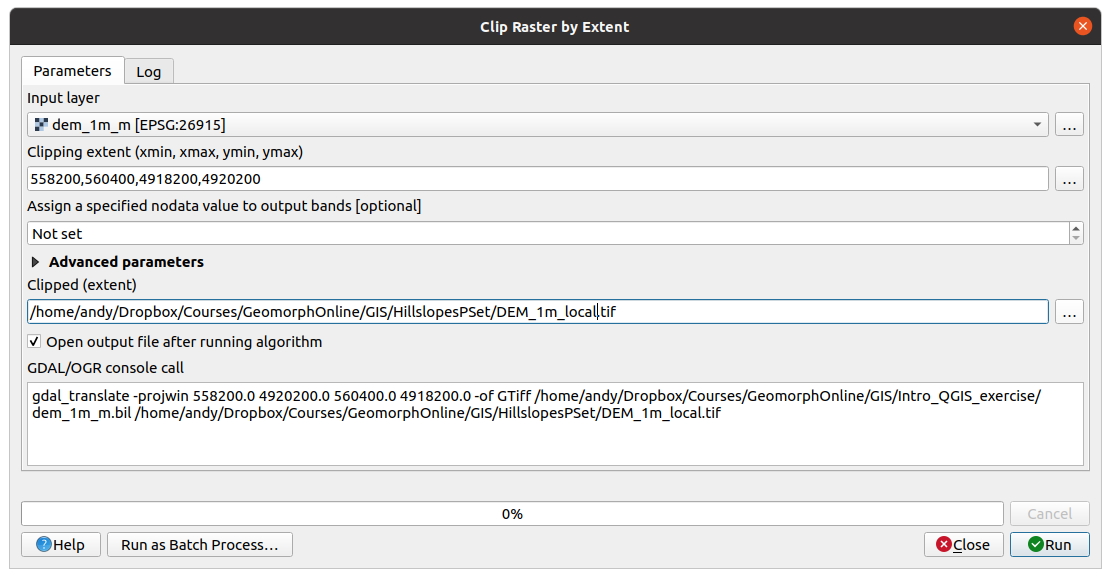
Bounding box: 558200,560400,4918200,4920200

Choose to save your output to a reasonable place on your computer (not to a temporary file unless you feel like losing your work) and hit “Run”.

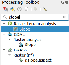
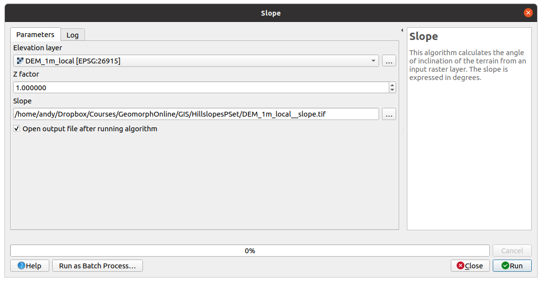
After this, use the built-in QGIS tool to compute the slope angle (in degrees):

Once you have completed this, use the “histogram tool” (also accessed via the processing toolbox) to compute a histogram and save it to an HTML file somewhere. (I’m not sure why QGIS saves this as a HTML, but it’s good enough for what we need it to do: visualize some data.) The x axis is the slope angle, and the y axis is the number of cells that fall within that angle.

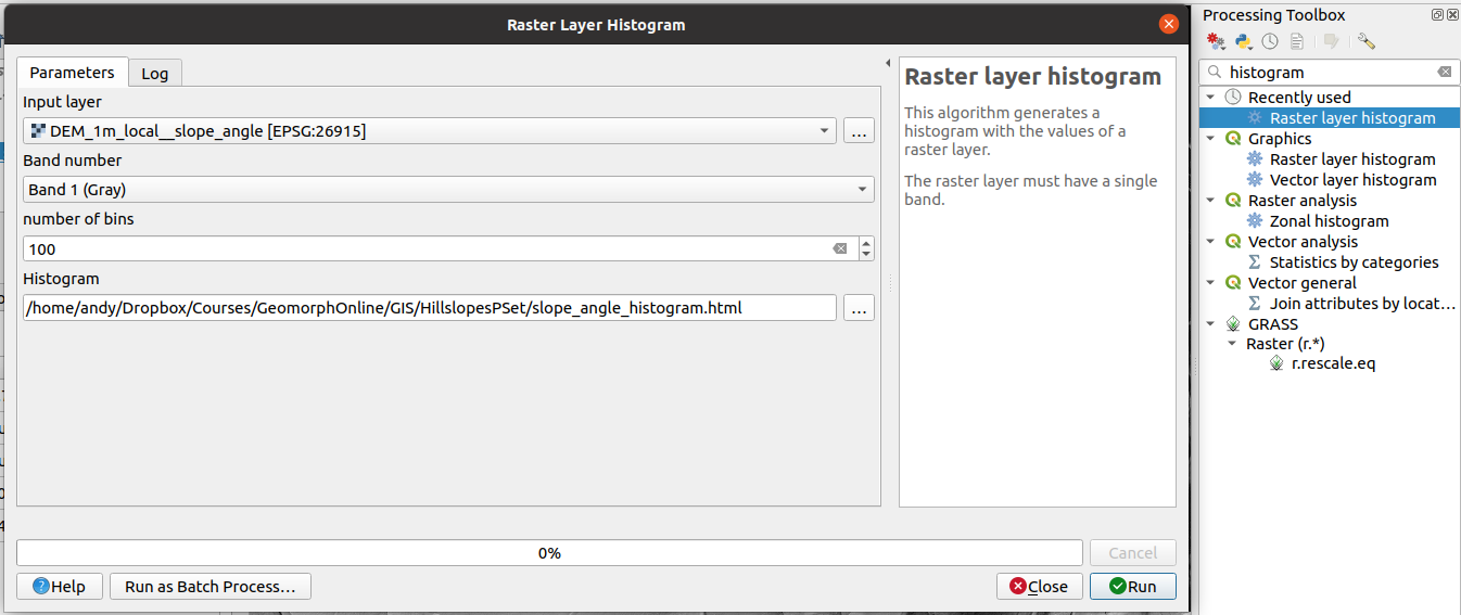
• Use 100 bins
• y axis: n cells
• x axis: bin (i.e., slope angle)

Computing the histogram might take some time, and it will get stuck on 99%. Don’t worry! Maybe do before making a snack / using the bathroom. Going on a jog works too, but it’s more a few minutes than a few tens, at least on my old-ish computer.

(b): 10 points: Why does this histogram look the way it does?

Why does the distribution of slopes on the DEM look the way it does? Think about different processes that could be intfluencing the topography. (Note: significant erosion has occurred in this region since the Mississippi River incised between ~2.5 and 0.8 million years ago: Over this time, the landscape has eroded on average.)

Take a screenshot of the histogram and annotate it, and write a paragraph supporting your conjectures. For example: Is the histogram continuous or not, and why? How does the set of slopes compare wtih the angle of repose, and is this as expected or is it surprising? Do you think that the slope map is more representative of channels or hillslopes? Can you see zones where gradual creep vs. sudden mass-wasting processes may be dominant? Support your ideas based on what we have learned about the mechanics of these landscapes.

3. Obtaining erosion rate and extent from hillslope diffusion and hilltop curvature (45 points)

In the geosciences, we often obtain rates from sets of dates – typically, radiometric dates. However, the topography also tells a story, and by interpreting it, you can also start to infer how quickly geological processes operate – and project into the future.

We’re going to start with the hillslope-diffusion equation in one dimension:

\[\frac{\partial z}{\partial t} = k_h \frac{\partial^2 z}{\partial x^2}\]

(a) 5 points: Dimensional analysis of hillslope diffusivity

\(k_h\) is the hillslope-diffusion coefficient, or “hillslope diffusivity”. Its numerical value is typically 0.05 (using time units of years and length units of meters… don’t want to give it all away!) for poorly-consolidated materials (e.g., glacial till, soils fine-grained sedimentary or metasedimentary rock). What are its units? Demonstrate this using dimensional analysis of the differential equation terms to the left and right of the “equals” sign.

Hint: the terms in the differential equation are really just giving you differences over an infinitesimally small distance. Remember that these have units! It might be helpful for your thinking to change the \(\partial\)s to \(\Delta\)s, or to entirely remove the derivative symbols (and to replace the letters with units).

(b) 15 points: Diffusion length

i: 5 points

Showing your work, use a similar approach to the dimensional analysis to show how you could intuit a how the characteristic horizontal (\(x\)) length scale of hillslope diffusion relates to the a time scale, \(t\). You can think of this length scale as the distance away from the channel that the hillslope has responded to river incision (or, if you prefer to personify a landscape, the distance over which the hills can “feel” the effects of the river). The time scale is the time since some sudden event, such as a rapid pulse of river incision. In the upper Mississippi valley, this pulse occurred sometime between 0.8 and 2.5 million years ago.

ii: 5 points

After writing this scaling argument, sketch half of a valley cross section, from the center line of the channel (your lowest point) and going perpndicularly out of the valley and towards the hills. Do so for three time steps, \(t_0\), \(t_1\), and \(t_2\). Hint: at your first time step, \(t_0\), you can draw the landscape as a sideways “L”, with a river that has cut a vertical slot canyon and the hill still being just a cliff. There is no need to have real values on the axes; the point is that you can intuit how hillslopes might respond to a sudden river incision over time.

iii: 5 points

The actual solution for this scaling (part i) is:

\(L = 2 \sqrt{k_m t}\),

where \(L\) is a characteristic length scale. Yes, I just gave you (sort of) the answer to this first part! And so this is why you have to show your work: I need to know that you know how you get to this length-scale–time-scale proportionality.

Considering that the bluffs of the upper Mississippi valley are made of dolostone, which is considerably less erodible than glacial till (though it can weather), I assume that:

\(k_m = 0.01\).

This value may be a bit high, but it sure makes the math easier!

The question for you: If it has been 2 million years since the Mississippi first incised, setting off hillslope diffusion, then how far from a channel might hillslope diffusion have reached in this time? How does this compare to the distances in the DEM subset that you used for Question 2? Based on this, would you expect that most regions between these valleys might be experiencing hillslope diffusion everywhere, or do you think that there could be some high plateaus that have not yet “felt” the river incision?

(c) 25 points: Solving for mean landscape erosion rate using hilltop curvature.

Let’s return to the hillslope diffusion equation:

\[\frac{\partial z}{\partial t} = k_h \frac{\partial^2 z}{\partial x^2}\]

We’ll make the simplifying assumption that the entire landscape – at least within the valleys and hills close to the Mississippi – is eroding at the same rate. Let’s call this rate \(\dot{\varepsilon}\), with \(\varepsilon\) standing for “erosion” and the dot indicating that it is a rate. Because this is steady in time and uniform in space, it is a constant.

\[\dot{\varepsilon} = k_h \frac{\mathrm{d}^2 z}{\mathrm{d} x^2}\]

By using this and analyzing the topography, you will be able to estimate the whole-landscape erosion rate.

i: 5 points

Mapping hilltop curvature

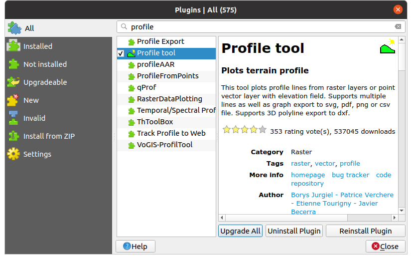
First, install the Profile Tool plugin from via the drop-down menu: Plugins → Manage and Install Plugins…:

Next, use the layer manager to import the line that I drew crossing a hillslope between two incising valleys.

Select this single line in the “layers” panel and open the Profiler Tool. Choose “selected layer” in the profiler tool for the source of the line, and add your DEM as the source for the elevation data.

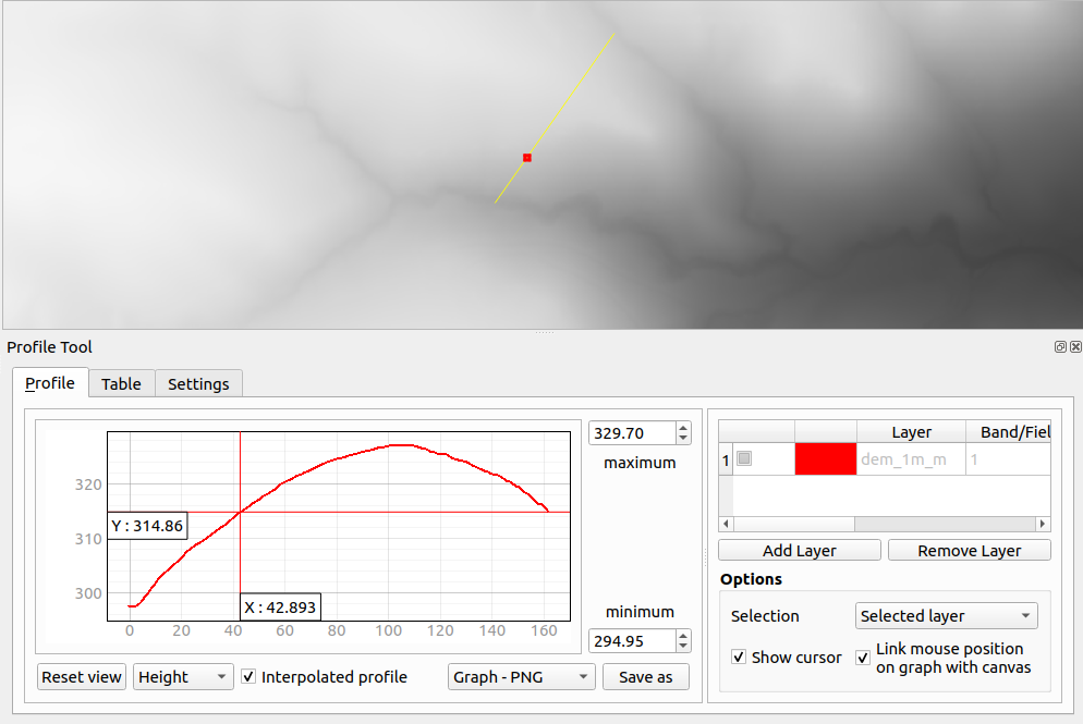
Take a screenshot of your computer at this stage to demonstrate that you have successfully extracted your own data. This will be the basis for the 5 points – basically, I want to give you some credit for griding through the mechanics of QGIS.

Then, go to the “Table” tab and copy the data table to the clipboard. This will contain \(x\) (distance along the profile) and \(z\) (elevation) data.

Paste this data set in your desired spreadsheet program. You are ready to begin the next step.

ii: 15 points

Solve for erosion rate

• First, create a plot of your data as a set of x,z points (or as a continuous line, your choice.
• Second, create a curve fit to this as a second-order polynomial
• Third, note that the parabolic fit, strictly speaking, is only valid near the top of the hill. Consider trimming some of the river valleys and surrounding regions. I expect you to obtain a good fit regardless, and for the result to be relatively insensitive to this.

Your mission now Once you have this fit, use it with the above equation to find the average erosion rate. For this, assume (as before), that \(k_m = 0.01\) in units of meters and years. When considering the sign of your solution, recall that erosion is defined such that down is positive. (Right? Becuase otherwise it wouldn’t be… eroding.)

Also: Project how much additional erosion might occur in the next 1 million years.

Turn in:

• A copy of your spreadsheet-generated plot with data, curve fit, and the curve-fit parameters (coefficients and goodness of fit
• Your computed average erosion rate, including your math/work to get there
• The estimated additional erosion after 1 million years of further hillslope evolution

iii: 5 points

You have solved for a natural backgorund erosion rate. Stan Trimble, geomorphologist from UCLA, studied erosion following Euro-American settlement in Coon Creek, a river basin on the Wisconsin side of the Mississippi valley. From his paper (linked here for those with UMN libraries access), he estimates an average depth of erosion of 13.2 cm over the course of time from 1853 to 1975, which encompasses the major phase of Euro-American settlement, land clearing, and unsustainable plowing practices.

Compare the natural erosion rate to the 19th–20th century rate, and (in a few sentences) and describe why you expect this discrepancy exists, perhaps drawing from some of the information you learned from Dave Montgomery’s lecture.

4. Identifying zones of likely mass-wasting processes in the landscape (30 points)

(a) 10 points: Comparing slopes to the angle of repose

Using the slope map that you built in Question 2, compute a binary raster based on slopes that are above the angle of repose (computed in Step 1). According to Byerlee’s Law, most geological materials have frictional properties that are similar to sand (\(\mu\) = 0.6). The best way to do this is by using the “Raster Calculator”, built in to QGIS. Produce a map with a descriptive legend as your output. Brownie points (but no real points) if you decide to create a nice-looking map with overlays or do something creative with the QGIS map composer.

(b) 5 points: Topographic observations

What do you notice that is different between the sections of the landscape that are above vs. below the anlge of repose? Describe this in ~2 sentences.

(c) 10 points: Cohesion

Regions of the landscape whose slopes are near or above the angle of repose can fail suddenly. Consider a 45-degree hillslope. What is the minimum cohesion (\(\sigma_c\)) that would be required to maintain this slope as barely stable (i.e., at incipient failure)?

Recall the general equation for slope stability (see the notes for more complete descriptions):

\[\tau = \mu \sigma_\mathrm{eff} \cos \theta + \sigma_c\]

along with the supporting equations for shear stress (\(\tau\)), which is the same as the driving stress (\(\sigma_d\), the stress pushing the system towards failure):

\[\sigma_d = \tau = \left((1 - \lambda_p) \rho_r + \lambda_p f_w \rho_w\right) g h \sin \theta\]

and the effective normal stress, \(\sigma_\mathrm{eff}\), which is part of the resisting stress term:

\[\sigma_\mathrm{eff} = \sigma - P_f = (1 - \lambda_p) \rho_r g h\]

Use the following parameters

• Slope angle \(\theta\) = 45 degrees
• Rock density \(\rho_r\) = 2840 kg/m\(^3\) (dolomite)
• Water density \(\rho_w\) = 1000 kg/m\(^3\) (dolomite)
• Porosity \(\lambda_p\) = 0.2
• Fractional pore content \(f_w\) = 0
• The coefficient of internal friction \(\mu\) = 0.6
• The thickness of the landslide block, \(h\) = 1 meter (roughly known due to the joint spacing in the bedrock)

Don’t forget to include units! For a better learning experience (but no extra credit), think about how much equivalent thickness of weight of water this cohesion represents, and think about that weight pushing in a way that holds the hillslope together.

(d) 5 points: Impact of rainfall on landslide hazard

What would happen to your perfectly balanced hillslope from part (c) if the water content in the rock, \(f_w\), increased? Show your work about which direction it would tip the stress balance. Would it make the hillslope more or less stable?

This work is licensed under a Creative Commons Attribution-ShareAlike 4.0 International License.