Problem Set: River incision, tectonics, and landscape evolution

Interactions between climate, tectonics, and Earth-surface processes set the form of landscapes.

Learning Goals

• Learn about the influence of tectonics, climate, and lithology on the longitudinal (long) profiles of bedrock (i.e., detachment-limited) river channels.
• Assess how the competition between bedrock-channel erosion (via fluvial processes) and hillslope diffusion set the location of channel heads, and discuss/predict how land-use changes may cause these to move.

River long profiles: Tectonic uplift and bedrock incision

You are studying a river draining a small mountain range along the eastern margin of the the tectonically active but never-glaciated tropical Andes. You have a time machine and a way of perfectly measuring elevations down river profiles, so you can directly link your observations to theory on how rivers should evolve over time. You’re going to look into how your study river changes, and think about what processes happened to cause it to look so different.

A few important characteristics of this river:

• It experiences the same precipitation rate at all elevations
• It is incising through the same type and strength of bedrock everywhere: Andesite, of course!
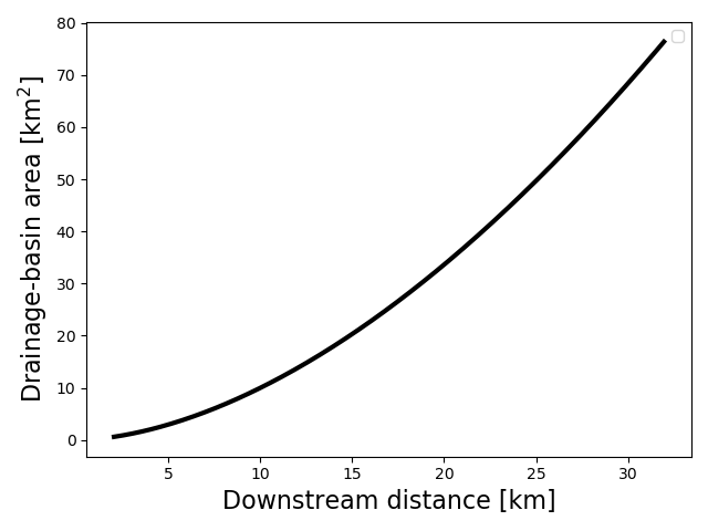
• Its drainage area increases downstream following Hack’s Law:

1. Detachment- and transport-limited river evolution (10 points)

In 1–2 sentences, describe the difference between detachment-limited erosion and transport-limited river-channel evolution. Then in another sentence or two, describe where you would expect each of these to dominantly occur.

2. The stream-power law (10 points)

Write out the stream-power law for detachment-limited erosion and describe the factors that impact its parameters.

3. Evolution of the river long profile

The plot below displays the long profile of a river, its elevation vs downstream distance along the river’s course, at multiple points in time. (This was created by me with the help of a little numerical modeling, but we’re still imagining that we’re in the Andes!)

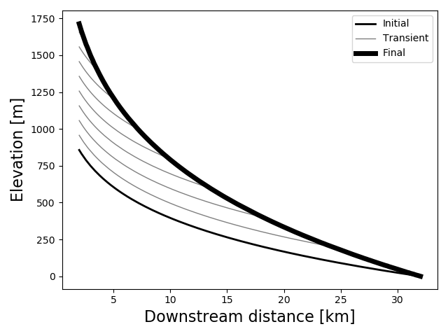
The river begins (thin black line) and ends (thick black line) at steady state, in which uplift equals erosion rate. During the interim, it is in a state of transience. “0” represents the base level, which you can consider to remain stationary over time, but does not represent any absolution elevation.

3.A (5 points)

What caused this change in the river long profile?

3.B (5 points)

During the time of adjustment, part of the channel has responded to the new conditions and part of the channel has not. Give the term for the geomorphic feature that connects the unadjusted portion of the river to the adjusted portion, and describe in a few words what this might look like in the field.

4. River profile concavity (5 points)

Both steady-state river long profiles are concave up. Based on the stream-power law for bedrock incision, why is this?

5. Concavity and steepness

A colleague with expertise in landscape analysis gives you a plot of the slope and drainage area of these channels.

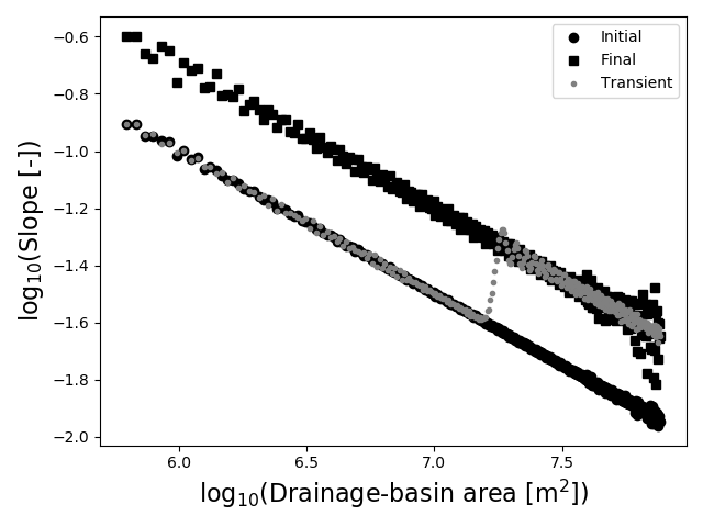
5.A (10 points)

By measuring / eyeballing this plot, provide the approximate \(k_s\) (steepness index) and \(\theta\) (concavity index) for both the initial and final long profiles. To start, you replot the data with enough space to draw the lines that you need to add for one of the two measurements.

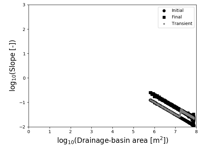
5.B (10 points)

Another local colleague tells you that she measured uplift rates and concavities in several regional streams and found that the stream-power erosion-rate coefficient, \(K\), should have a value of \(1 \times 10^{-6}\). Your stream has a similar lithology and climate. Based on this information and your measured \(k_s\), quantify the change in the external driver (which you identified in 3.A) that drove the river’s adjustment from the initial to the final long profile. To do so, provide this value for both the initial and final profiles, and comment on its magnitude of change.

6. Climate impacts (10 points)

Imagine a different future that it becomes much drier. How would this affect the stream-power erosion coefficient, \(K\), and the steady-state height of the mountain range?

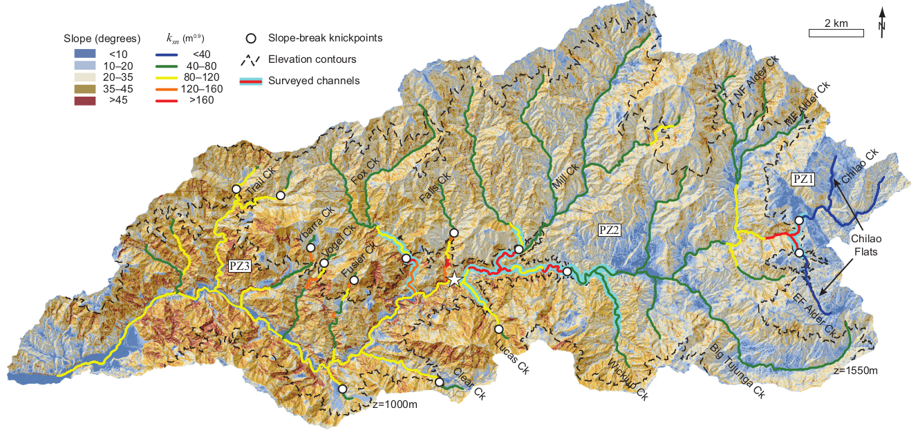
7. Faults in the landscape (10 points)

Based on what you know about both hillslope and fluvial processes, draw a straight line across this map that you think should represent the dominant fault. Note that \(k_{sn}\) is a concavity-normalized version of \(k_s\), but that it provides essentially the same information as that which you were analyzing above. Make a note of where you think that relative uplift rate is higher vs. lower across this fault. (You may want to open the figure in a new tab to get a big version.)

I’m not referencing the paper to keep the location (and answer!) sort of secret for the sake of the assignment, but anyone concerned about attribution can indeed contact me. This is from a colleague’s published scientific paper.

This work is licensed under a Creative Commons Attribution-ShareAlike 4.0 International License.