Hack’s Law, channel concavity, the steepness index, and river-profile analysis

We can decribe river and drainage basin geometry in a way that links to the stream-power law for bedrock incision.

Learning Goals

• Learn how drainage-basin area and river discharge relate via Hack’s Law.
• Know the definitions of steepness and concavity index for river systems.

Hack’s Law

Hack’s Law relates river-channel length, $l$, to drainage area, \(A\). It might be obvious that a longer river should necessitate a larger drainage basin!

\[l \propto A^h\]

Here, \(h\) is Hack’s exponent, and commonly has a vlaue of 0.5–0.6. Let’s think about the shapes of drainage basins that would cause Hack’s exponent to be small vs. close to 1.

Hack (1957) defined the drainage-area-to-mainstem-channel-length relationship. For more information, check out the Topo Toolbox blog post

The exponent, \(h\), is obtained by a curve fit with data from natural landscapes.

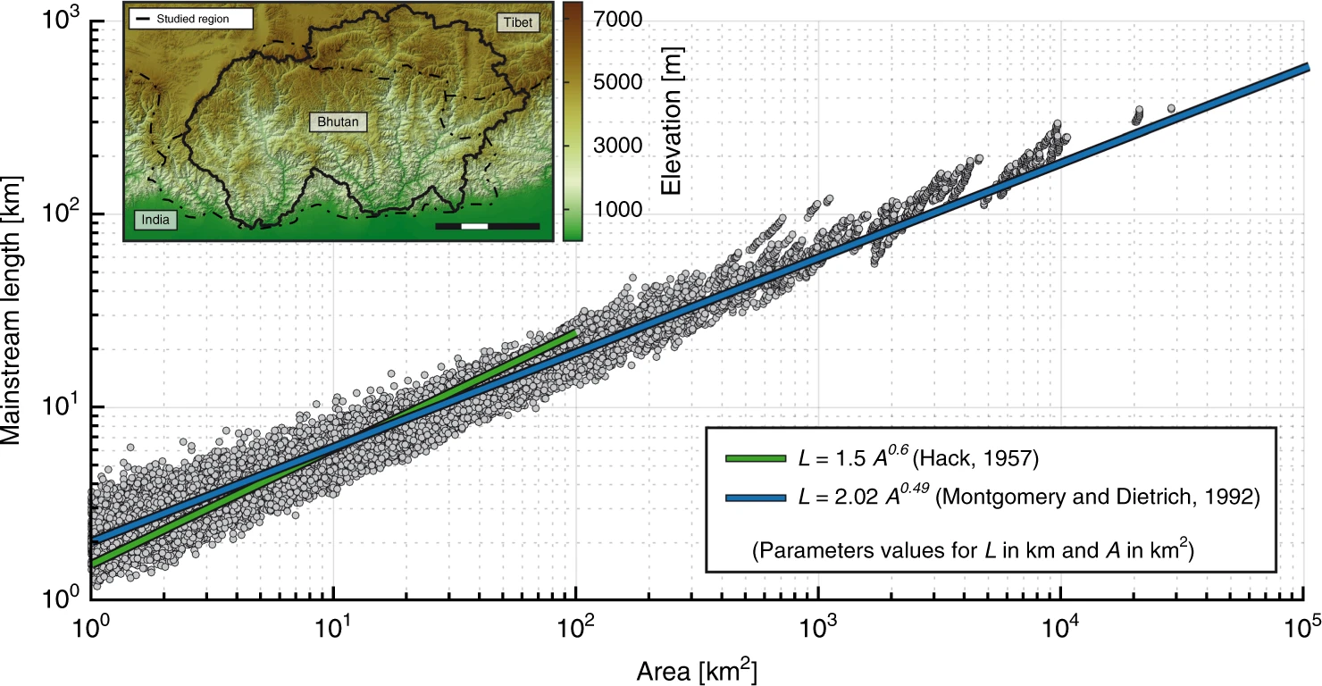
Hack’s Law describes the relationship between the length of the longest river in a catchment and the drainage-basin area. This data set from Sassolas-Serrayet et al. (2018) shows how it holds true across the Bhutanese Himalaya.

Rivers in more humid climates tend to be fed by more groundwater, leading to wider angles between tributaries. This leads to broad, branching drainage networks and a greater increase in dranage-basin area than in arid systems, which are fed by overland flow that produces river systems that flow more parallel to one another.

From Yi et al. (2018).

Channel steepness and concavity

Most channels have a concave-up long-profile shape, but even if they don’t, it is useful to find a way to characterize their concavity. In terms of downstream coordinates, one might characterize channel concavity in terms of the \(x\) (downstream) and \(z\) (bed elevation) coordinates as:

\[\text{Concavity} = \frac{\mathrm{d}^2 z}{\mathrm{d} x^2}.\]

However, geomorphologists define a separate concavity index that relates to drainge-basin area, which as you now know, also relates to distance downstream. We define a slope–area relationship as:

\[S = k_s A^{-\theta}.\]

Here, \(S\) is channel slope, \(k_s\) is a steepness index, and \(theta\) is the concavity index.

Steepness index indicates whether a channel is unexpectedly steep or gentle in slope when compared to its drainage area. We expect channel slopes to decrease wtih drainage-basin area.

Concavity is positive for a concave-up channel, negative for a convex-up channel, and 0 for a channel with a constant slope. (I can write this because of the Hack’s Law relationship between channel distance downstream and channel concavity.)

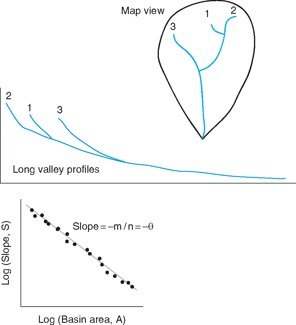
This figure, reproduced from the Anderson & Anderson Geomorphology textbook, shows the relationship between drainage-basin area, slope, and concavity. The log of channel steepness index would be the \(y\) intercept on this plot. To see how this works, take the log of both sides of the equation above.

Steepness and river long profiles

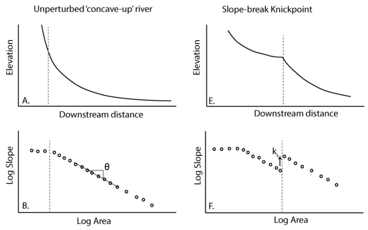
Modified from Boulton et al. (2013)

• The slopes of hillsides and debris-flow channels are unchanging with respect to drainage area. Panels A and B indicate this.
• A knickpoint – a sudden break (increase) in slope in the river long profile, is represented by an increase in the steepness index. Such a knickpoint may represent a different lithology or climate or the response of a river to some tectonic uplift event.

Steepness, uplift, and stream power

The stream-power law has a similar form to the slope–area relationship that defines channel concavity:

\[\dot{\varepsilon} = K A^m S^n.\]

Recall that \(\dot{\varepsilon}\) is vertical erosion (i.e., incision) rate, and that \(K\) is erodibility (related primarily to lithology, climate, and hydrology).

Let’s turn this into a landscape-evolution equation by including tectonic uplift, \(U\):

\[\frac{\mathrm{d} z}{\mathrm{d} x} = -K A^m S^n + U.\]

We’ll next posit that we are at topographic steady state: that is, erosion equals uplift everywhere:

\[U = K A^m S^n.\]

With some algebra, we can rearrange this into a form similar to that of the slope–area relationship:

\[\frac{U}{K} = A^m S^n\] \[S^n = \frac{U}{K} A^{-m}\] \[S = \frac{U}{K} A^{-m/n}\]

The finding here is profound.

The concavity index is equal to \(m/n\), and tells us about these terms in the stream-power erosion law.

\[\theta = \frac{m}{n}\]

The steepness index increases with uplift rate and decreases with erodibility. Rapidly uplifting hard rock requires the steepest channels to erode at a pace that is comparable to the rest of the river system.

\[k_s = \frac{U}{K}\]

Therefore, we expect knickpoints, steep zones in rivers, to occur where rocks are hard and/or tectonic uplift is fast.

If we also have a geological map, we can control for the effects of lithology, and thereby relate river-profile shapes to rates of tectonic uplift.

Finding the concavity and steepness indices from a log–log plot

Above, we showed that we can learn something about landscape evolution and bedrock incision from river long profiles and their steepness indices and concavity indices. But how do we find these terms from a set of data? Let’s go back to the equation that describes channel long-profile shape.

\[S = k_s A^{-\theta}.\]

We can measure slope (\(S\)) and drainage area (\(A\)). There remain two parameters to fit.

By taking the log of both sides of the equation, we can make inroads into turning it into a linear form:

\[\log_{10}(S) = \log_{10} \left(k_s A^{-\theta} \right).\]

From rules of logarithms:

\[\log_{10}(S) = \log_{10}(k_s) - \theta \log_{10}(A).\]

This has the form of our very old friend from algebra, \(y = mx + b\), with a \(y\)-intercept of \(\log_{10}(k_s)\) and a slope of \(-\theta\).

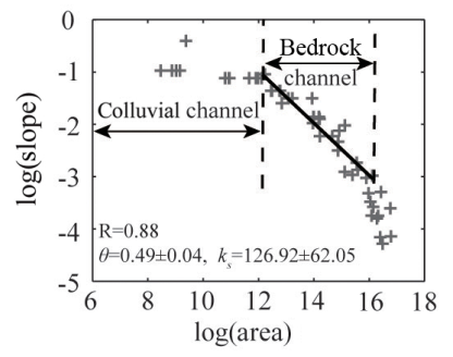
In the figure above, Wang et al. (2017) analyze the concavity and steepness of a river along the tectonically active California coast. Their “colluvial channel” here represents the hillslopes and associated processes of creep, landslide, and debris flow. These are logarithmic axes, and demonstrate how one would fit the slope and \(y\) intercept to obtain \(-\theta\) and \(k_s\), respectively.

This work is licensed under a Creative Commons Attribution-ShareAlike 4.0 International License.